TL;DR: Once you can read Throughput, you can use it for probabilistic forecasting. Monte Carlo Simulation turns historical completed work into ranges, percentiles, and a better conversation about delivery risk.

This is a follow-up to the Throughput article. If you need the foundation first, start with Throughput: the flow metric behind team predictability. Here I will not re-explain the metric. Here we turn historical completed work into a forecast.
Now let’s get to the practical question management loves to ask: “When will this project of X items be done?”
What Monte Carlo Forecasting Answers
Teams usually need three forecasts.
- When will we finish X items? For example, an epic with 10 work items.
- How many items can we finish by a date? For example, what is realistic by the end of the quarter.
- How much work should we pull into the next sprint, week, or month? Capacity becomes a probability conversation, not a negotiation around estimates.
All three use the same idea: take the history of completed work, sample from it many times, and see which futures appear most often.
Before You Simulate
Check the system before trusting the graph.
- Definition of Done is clear. Closed means done, not moved to a different waiting room.
- The workflow is stable enough. The team, process, and work type have not changed radically in the last few weeks.
- The historical window is fresh. Three to six months is usually enough. Older data often describes another system.
- Zero-throughput days are preserved. Weekends, holidays, sick days, and no-release days are part of reality.
- WIP is limited at least by an upper bound. Without a cap on unfinished work, the forecast becomes a nice chart on top of chaos.
- Items are not closed in artificial batches. Backdated batch closing creates fake throughput spikes.
Monte Carlo will always draw a distribution. The question is whether that distribution describes delivery risk or just the mess in the data.
Foundations of Probability-Based Forecasting
Any forecast always involves 3 essential bits:
Probability
Spread
Assumption that future work resembles historical patterns
Saying “This epic (10 tasks) will take exactly 6 weeks” is misleading. A more accurate forecast: 10 tasks in 5–7 weeks, where:
5 weeks = 50th percentile (half of runs finish by then)
7 weeks = 85th percentile (85% of runs finish by then)
How Monte Carlo Simulation Works
Disclaimer: Here and further on I’ll be using charts built with Predictable.team (my vibe-coded react app that visualises and forecasts team performance based on Jira / Youtrack CSVs).
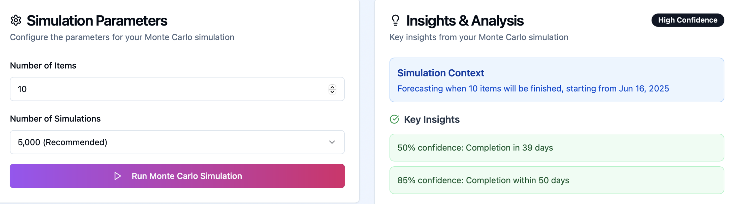
Let’s imagine that we need to understand when will the next 10 items be ready.
1. Collect historical throughput data
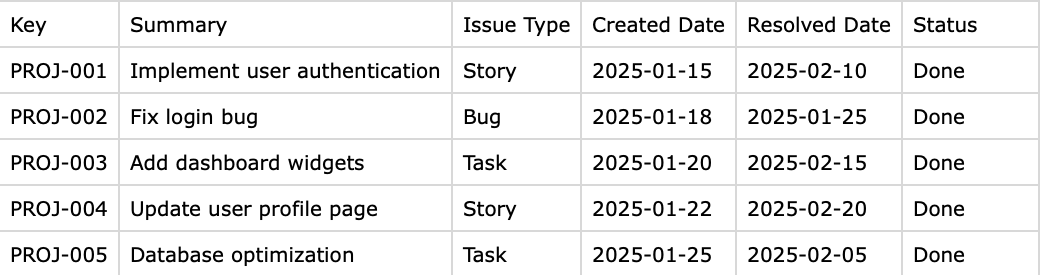
Imagine you have information about how many items your team finishes every day for a consistent period of time. Always count all days, including the ones with 0 deliveries.
Let’s say our dataset is 90 days. A random number should be generated in the range from 1 to 90, because each of those randomly generated numbers represents a day from that dataset.
2. Run 1,000–10,000 simulated scenarios. For each simulation (code sample below):
- Generate random number.
- This random number will represent a day from our stats (one of those 90).
- Record how many items have been delivered during that day
- Let's say we got 20, and on 20th day from our dataset we've delivered 1.
That means that so far we have 1 item delivered.
Continue generating random numbers until you get 10 (since we wanted to know when we’ll deliver next 10 items).
Voila, your first scenario is ready. Thousands more to go!
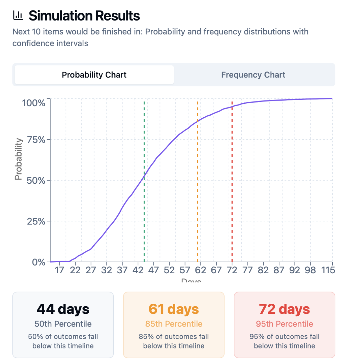
3. Display a probability distribution of completion times
- Take a look at 50th pp (50% of simulations had 10 items be finished at this number of days or less).
- You can plan at 50th pp as long as you have WIP limits and control aging within your system.
- Take a look at 85th pp (85% of simulations show that 10 items would be delivered by that day)
- 85th pp is a conservative estimate, which strikes great balance between risk and speed.
- You can also forecast saying 50pp-85pp as a range, since all forecasts have range, probability and assumption that our work would be similar in the future.
Example for 10 tasks:
50% probability: 39 days
85% probability: 50 days
95% probability: 58 days
Present to stakeholders: “Forecast: it will take 39-50 days.” Using the 85th percentile offers a safer buffer, though planning at the 50th percentile is common practice.
Higher throughput stability (lower variation) means the 50th and 85th percentiles converge, tightening the forecast.
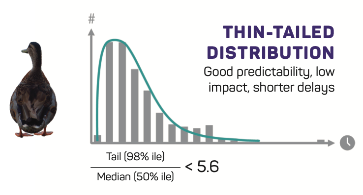
As per David Andersen, proper predictability is 98pp/50pp < 5.6
Factors Affecting Forecast Quality
Task breakdown: End-to-end slices yield better forecasts than component-only slices.
Historical window: Avoid using data older than six months.
Zero-throughput days: Include them to reflect weekends, holidays, sick days.
Calendar vs. work days: Always use calendar days to account for non-working periods.
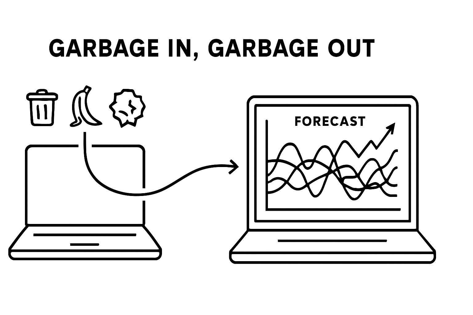
Also: Garbage-in, Garbage-out. If your data is bad, not full
WIP is essential for reliable forecasting
Monte Carlo forecasts require enforced WIP limits. As Daniel Vacanti warns:
“No WIP limit = no flow, which means no predictability.”
Forecasting should always be updated
Run fresh simulations every 1–2 weeks to adapt to changing conditions. Just like during weather forecasts on forest fires, earthquakes, traffic forecasts and other systems, we can’t and never will account for all parameters in the equation, hence we need to update our forecasts using our latest data.
Are there better models than just random MCS sampling?
Prateek Singh of ActionableAgile made a research proved that explained here “random” method actually produces the best forecasting results compared to more sophisticated day-matching algorithms.
You can read the research at the link above or watch recent their episode of Drunk Agile (kudos for the guys on that name):
https://www.youtube.com/watch?v=gO3Uw7CG04I
Why Throughput Works
By the law of large numbers, sufficient throughput history smooths out random variation in work size and type, converging on a stable average performance metric.
That’s applicable not only in relying on Throughput and forecasting via MCS (Monte-Carlo Simulation), but thinking about outcomes of you DnD fights :)

Nifty things
Monte-Carlo Forecasting tools
Predictable Team - safe stateless web app. Ingests CSV / XLSX from jira and youtrack. Visualizes Throughput from the file + performs Monte-Carlo Simulation based on your data (When will be project finished, how many items to take in a sprint, when will the epic be done).
TWIG from Actionable Agile. Super-awesome app that is de-facto industry standard together with getNave. Visualizes metrics + does MCS.
Some reading references
“Monte Carlo Simulation Analysis of Team Strategies and Backlogs” - Matthew Croker, 2023 - Replication study of Prateek Singh’s experiment using 10,000 simulations, showing specialized strategies deliver faster short-term results but generalized approaches prove more effective long-term.
** **“All Models are Wrong, but Some are Random…” - Prateek Singh, 2021 - Back-testing study comparing five different Monte Carlo sampling models, proving simple random sampling consistently outperforms Markov chain and weekday-matching approaches.
“Agile project status prediction using interpretable machine learning” - Forouzesh-Nejad et al., 2023 - Achieved 97% accuracy in agile project forecasting using team throughput data, significantly outperforming traditional methods.
“Empirical findings on team size and productivity in software development” - Rodríguez et al., 2012 - Large-scale empirical study with 195+ citations analyzing team productivity factors critical for throughput-based forecasting accuracy.